Implementation of Linear Predictive Coding (LPC) for Speech Synthesis
Created by Corinne Darche for MUMT307: Music and Audio Computing II (Winter 2022)
Project Description: What is LPC?
Linear Predictive Coding (LPC) is a method for analyzing signals quickly and accurately. As described by O’Shaughnessy (1998), LPC’s main draw is that it can accurately estimate vocal fold vibration, the vocal tract’s shape, and the different vocal tract resonances. Sawant et al. (2010) went on to explain that LPC’s technique predicts a small number of coefficients, which represent different speech parameters, that are then applied in digital filters to create a synthetic version of the original speech signal.
This Matlab script implements a version of the LPC algorithm to analyze and resynthesize an audio file, either with real-time I/O, pre-recorded and saved files, or a combination of the two.
Project Goals
- Learn more about speech synthesis.
- Most of my experience with language processing has been through the lens of text-based NLP, so this is a natural next step.
- From the title of this course, this class mostly focuses on pitched sounds. However, if you take a look at the literature surrounding singing voice generation and analysis, the roots come from speech processing. Singing generation and analysis is still a huge challenge and research topic in sound synthesis, so a strong understanding of speech generation concepts is a must.
- Continue to explore Matlab’s full programming capabilities
- Learn more about Linear Predictive Coding
- It’s one of the most popular speech synthesis algorithms for a reason.
Methodology and Design
The script follows a basic implementation of the LPC algorithm. I started off using an implementation described in Matlab’s DSP Toolbox documentation. However, I wanted to use as little of the toolbox as possible, since it’s a black box and it would hinder the learning experience.
There are three main features that can be toggled by user input: audio input, audio output, and spectrum analyzer.
This script gives the user the option to either provide their own pre-recorded audio file or to record up to 5 seconds of speech audio using their computer microphone. I provided two audio inputs, “example.m4a” and “differentLevels.m4a”, as test audio inputs. The real-time input is then saved as “LPC_input.m4a” and then passes through the LPC algorithm, similar to a pre-recorded file. This was adapted from the reference in the Matlab documentation.
The user is also prompted to select whether they want the output to play in real-time or to save it as a .m4a file. If the output is saved, the user is told that it is saved to a file called “LPC_output.m4a” within the same folder as the script.
The user is also prompted to turn on or off the spectrum analyzer, a visual support for the LPC synthesis. They are able to view the speech signal alongside the curve produced by the computed coefficients from the Levinson-Durbin algorithm. Note that this feature does slow down the runtime.
The LPC algorithm can be divided into different sections. The complete audio file is divided into frames (defined in the script as 1600) that the algorithm goes through one by one during the analysis before recombining them during the resynthesis. First, there’s pre-emphasis, where the signal is filtered to give it a smoother spectral shape. This is done using a simple FIR filter with the difference equation y[n]=x[n]−ax[n−1] where 0.9<a<1.0. The audio quality of the final synthesized version decreases as the value of a decreases. Then, the signal passes through a Hamming window to further smooth it for analysis. It then passes through a 12th order autocorrelation sequence. Autocorrelation is the correlation of a signal with a delayed version of itself, and it is a tool used to find repeating patterns. The autocorrelated signal is then sent through the Levinson-Durbin algorithm to determine its reflection coefficients and error.
The pre-emphasized signal and the resulting Levinson-Durbin coefficients are then passed through two lattice filters: one is a FIR lattice filter and the other is an IIR filter. This reconstructs the original signal frame by frame for output. Taken from the Matlab documentation, there is also an option to view the scope of the signal as well as the curve generated by the LPC coefficients.
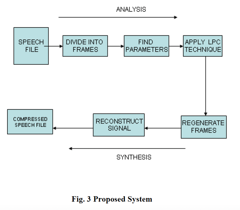
Diagram of LPC analysis and resynthesis, as seen in Sawant et al. (2010)
Discussion (Challenges, Successes, etc.)
This was a challenging subject to learn as an “outsider”. A lot of the resources that I tried to use assumed that I had a strong background in the subject and jumped straight into a lot of mathematical theories. Sources that did show an implementation, like Matlab’s MathWorks documentation, did it in a black-box method. That is, there was no way to see what exactly was happening underneath those functions. Yes, the implementation worked, but I had no idea what they did exactly to get to that finished product. This meant that I had to get creative and do some extra reading and digging to figure out how to implement this on my own.
Most of the literature that I found insisted on using a Hamming window to smooth out the signal. Based on what we’ve learned about windowing techniques, it’s a logical choice since it smooths out the envelope and doesn’t create a sharp ending on any of the frames. To further confirm my understanding, I tried swapping it out for a rectangular window or a triangular window, only to find that the output would get abruptly cut off before the end of the input file. Hanning and Blackman windows served as good substitutes for the Hamming window, since they have a similar spectra (see Week 6 notes).
In my initial plan, I wanted to create a Graphical User Interface (GUI) for the script and turn it into a proper application. However, Matlab’s GUI is awkward to use. The only option was to create a live script, but the formatting options did not fit the vision that I had in my head. I also wanted to focus less on creating a nice UI and stick to the main objectives of this project. As such, a simple Matlab script with user input at runtime ultimately served my project’s purpose better than Matlab’s GUI.
LPC’s primary objective is to reduce the bit-rate of the final resynthesized file. However, when seeing my implementation, I notice that my generated files are significantly larger than my pre-recorded ones. There is a possibility that Apple’s algorithm for creating .m4a files on “Voice Memos” is significantly more space efficient than my LPC algorithm. It may be more useful to use “.wav” files rather than “.m4a” files to fully view LPC’s compression.
Conclusions and Future Work
This project allowed me to explore a specific speech synthesis algorithm at the forefront of speech processing. I successfully implemented the algorithm and created a practical script for users to experiment with. While MATLAB’s shortcomings made me adjust my project, I still maintained my previously mentioned goals.
In future work, I would like to keep exploring different speech synthesis techniques beyond LPC. I could look into formant-based synthesis and even machine learning methods for speech synthesis with Hidden Markov Models and Deep Learning. I would also like to add more features to this script specifically, like pitch bending. To get the GUI that I want, I would have to transfer this project off MATLAB into a different programming language, such as C++ or Python.
References
MathWorks. 2022. “LPC Analysis and Synthesis of Speech.” MathWorks. Accessed April 7, 2022. https://www.mathworks.com/help/dsp/ug/lpc-analysis-and-synthesis-of-speech.html.
MathWorks. 2022. “Record from sound card.” MathWorks. Accessed April 9, 2022. https://www.mathworks.com/help/audio/ref/audiodevicereader-system-object.html.
O’Shaughnessy, Douglas. 1998. “Linear Predictive Coding.” IEEE Potentials 7 (1): 29-32.
Sawant, G., A. Singh, K. Kadam, R. Mazarello, and P. Dumane. 2010. “Speech Synthesis Using LPC.” In Proceedings of the International Conference and Workshop of Emerging Trends in Technology, 515-517.